The best way to learn is learn the fundamentals. This hands-on approach allowed me to grasp essential concepts, understand the inner workings of neural networks, and appreciate the complexity and beauty of machine learning. In this journey, I not only built a functional library but also gained invaluable knowledge and experience.

To learning machine learning fundamentals, I create my own neural network library “mikir” from scratch and the project available in GitHub!

So, let get started on walkthrough how I made it.

Neurons concept

The first thing that come to neural network and machine learning is neuron. It’s inspired by biological neurons in the brain. In biology, neurons receive signals, process them, and transmit the result to other neurons.

Components of an artificial neuron

• Inputs: these are the incoming signals, often outputs from other neurons or intial data.
• Weights: each input has an associated weight, indicating its importance.
• Bias: an additional parameter that allows the neuron to shift its activation function.
• Summation Function: Combines all weighted inputs and the bias.
• Activation Function: Determines the neuron’s output based on the summation.

How neuron works

• It receives inputs
• Each input is multiplied by its corresponding weight
• All weighted inputs are summed together, and the bias is added
• This sum is passed through an activation function to produce the output

Understanding weight and biases

These two are confusing concept if you dont have solid example. So let’s break them down:

Weights determine strength of the connection between neurons. They multiply the input values, increasing or decreasing their importance. During training, weights are adjusted to make network’s predictions more accurate. Think of weights like the importance you give to different factors when making a decision.

Bias allows the neuron to shift its activation function left or right. Adding to the sum of weighted inputs before the activation function is applied. Like weights, biases are adjusted during training. Think of bias as threshold that the weighted sum needs to overcome to “activate” the neuron.

Let’s use simple example to illustrate:

imagine a neuron that decides whether to recommend an ice cream flavour based on two inputs: temperature (in Celcius) and your hunger level (on a scale of 0-10).

class IceCreamNeuron {
    constructor() {
        this.weightTemperature = 0.7;  // Temperature is quite important
        this.weightHunger = 0.3;       // Hunger is less important
        this.bias = -15;               // You need some convincing to eat ice cream
    }

    recommend(temperature, hungerLevel) {
        const weightedSum = (temperature * this.weightTemperature) + 
                            (hungerLevel * this.weightHunger);
        const activation = weightedSum + this.bias;
        
        // Simple step function instead of sigmoid for this example
        return activation > 0 ? "Yes, eat ice cream!" : "No, skip the ice cream.";
    }
}

const iceCreamDecider = new IceCreamNeuron();

console.log(iceCreamDecider.recommend(30, 8));  // "Yes, eat ice cream!"
console.log(iceCreamDecider.recommend(15, 2));  // "No, skip the ice cream."

In this example:

1. Weights: temperature has a higher weight than hunger, meaning it influences the decision more.
2. Bias: the negative bias means that the weighted sum needs to be at least 15 for the neuron to recommend ice cream. This could represent a general reluctance to eat ice cream unless conditions are really favorable.
3. Decision making:

• On hot day (30C) when you’re quite hungry (8/10), the neuron recommends ice cream: (30 * 0.7) + (8 * 0.3) - 15 = 23.4
• On a cool day (15C) when you’re not very hungry (2/10), it doesn’t: (15 * 0.7) + (2 * 0.3) - 15 = -3.9

In neural network, these weights and biases are adjusted during training to make better predictions. For instance, if this neuron consistently recommended ice cream when it shouldn’t, the training process might decrease the weights or lower the bias to make it “more conservative”.

Activation function

The activation function introduces non-linearity, allowing neural network to learn complex patterns. Common activiation functions include:

• Sigmoid: maps input to a value between 0 and 1. Useful for predicting probabilities.
• ReLU (Rectified Linear Unit): returns 0 for negative inputs, and the input value for positive input.
• Tanh: similiar to sigmoid, but maps to values between -1 and 1.

What does it mean to be non-linearity

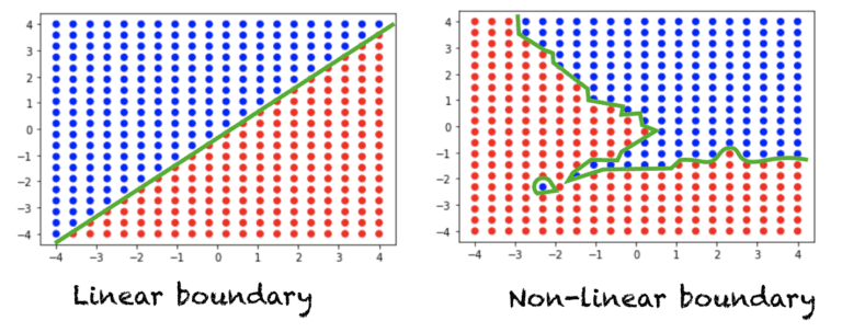
• A linear function is a straight line when graphed. It has the form y = mx + b.
• A non-linear function produces a curve or any shape that’s not a straight line when graphed.

Let’s illustrate this with some examples:

Linear example: Temperature conversion Fahrenheit to Celsius: C = (F - 32) * 5/9

This is linear because it’s a straight line when graphed Every 9°F increase always results in a 5°C increase

Non-linear example: Compound interest A = P(1 + r)^t, where A is the final amount, P is principal, r is interest rate, t is time

This is non-linear because it curves upward when graphed The growth accelerates over time, it’s not constant

For instance, in image recognition, the relationship between pixel values and the object in the image is highly non-linear. Non-linear activation functions enable neural networks to capture these complex patterns.

This broader predictive capability is why neural networks with non-linear activation functions are so powerful. They can approximate a wide variety of functions, allowing them to model complex relationships in data that linear models simply cannot capture.

Implement basic neuron

Now, let’s implement a basic neuron class to illustrate these concepts:

class Neuron {
    public weights: number[]
    public bias: number

    constructor(inputCount) {
        this.weights = new Array(inputCount).fill(0).map(() => Math.random());
        this.bias = Math.random();
    }

    activate(inputs) {
        const sum = inputs.reduce((sum, input, index) => sum + input * this.weights[index], 0);
        return this.sigmoid(sum + this.bias);
    }

    sigmoid(x) {
        return 1 / (1 + Math.exp(-x));
    }
}

module.exports = { Neuron };

Let’s break down this implementation

1. Constructor:

• I love defined and book variables in class, we defined weights as array of number and bias as number
• Initialized weights and bias with random values between 0 and 1 using Math.random
• The number of weights matches the number of Inputs

2. Activate method:

• This is the summation function.

1. sum variable multiplies each input by its corresponding weight and sums the results

2. the bias is added to sum

3. Sigmoid method:

• This is the activation function.
• It takes the big sum and maps it to value between 0 and 1 using sigmoid formula
• The sigmoid function is useful because:

1. It introduces non-linearity, allowing the network to learn complex patterns
2. Its output can be interpreted as a probability
3. It has smooth gradient, beneficial for learning

By the end of the process, our goal is to feed neuron either from input or another neuron’s output, process it and produce output to be feed to other neuron or make a decision (classify) from between 0 and 1.

Neural network components

• Input layer: receives intial data
• Hidden layer(s): processes information
• Output layer: produces final results
• Learning: adjusting weights and biases to improve predictions, often uses backpropagation and gradient descent

Every layer has bunch of neurons. Each neuron or nodes receives inputs, applies weights and biases, and produces an output

Neurons are connected between layers. Each connection has an associated weight.

Forward propagation vs Backpropagation

Forward Propagation:

Purpose: To generate predictions or outputs from input data. Direction: Moves from input layer through hidden layers to output layer. Process:

• Takes input data and feeds it through the network.
• At each neuron, computes weighted sum of inputs and applies activation function.
• Passes results to the next layer until reaching the output.

When used: During both training and inference (prediction). In the code: Implemented in the predict method.

Backpropagation:

Purpose: To train the network by adjusting weights and biases. Direction: Moves backwards from output layer through hidden layers to input layer. Process:

• Calculates the error at the output layer.
• Propagates this error backwards through the network.
• Computes gradients to determine how each weight contributed to the error.
• Updates weights and biases to minimize error.

When used: Only during training, not during inference. In the code: Implemented in the train method.

Key Differences:

1. Purpose: Forward propagation makes predictions, backpropagation improves those predictions.
2. Direction: Forward propagation moves forward through the network, backpropagation moves backward.
3. Calculation: Forward propagation calculates outputs, backpropagation calculates gradients and errors.
4. Timing: Forward propagation happens first, followed by backpropagation during training.

You’ll see forward propagation on predict and train method and backpropagation on train method after forward propagation. See the implementation section later.

Error Calculation

Error calculation is the process of determining how far off the network’s predictions are from the actual target values.

const outputErrors = outputs.map((output, i) => {
    const error = targets[i] - output
    return error * output * (1 - output)
})

This code calculates the error for each output neuron:

targets[i] - output is the raw error (difference between target and prediction). error * output * (1 - output) is the error gradient, using the derivative of the sigmoid function.

Weight Updates

Weight updates are how the network “learns” from its errors. The general formula is: new_weight = old_weight + learning_rate * error * input

neuron.weights = neuron.weights.map((weight, j) => {
    return weight + learningRate * outputErrors[i] * hiddenOutputs[j]
})

This updates each weight based on:

1. The current weight value
2. The learning rate
3. The calculated error
4. The input that contributed to this error (hiddenOutputs[j] for output layer, inputs[j] for hidden layer)

Learning Rate

The learning rate (often denoted as η or alpha) determines the step size at each iteration while moving toward a minimum of the loss function.

Key points about learning rate:

• A high learning rate can cause the model to converge quickly but may overshoot the optimal solution.
• A low learning rate leads to slower learning but can find more precise solutions.
• It often requires tuning to find the optimal value for a specific problem.

Epochs

These three elements work together in the learning process:

Forward propagation produces an output. Error calculation determines how far off this output is from the target. Backpropagation distributes this error back through the network. Weight updates adjust the network parameters to reduce this error. The learning rate controls how big these adjustments are.

This process repeats for many examples (often called epochs), gradually improving the network’s performance.

Implement neural network

import Neuron from './neuron.js'

class NeuralNetwork {
    private hiddenLayer: Neuron[]
    private outputLayer: Neuron[]

    constructor(inputCount: number, hiddenCount: number, outputCount: number) {
        this.hiddenLayer = new Array(hiddenCount).fill(null).map(() => new Neuron(inputCount))
        this.outputLayer = new Array(outputCount).fill(null).map(() => new Neuron(hiddenCount))
    }

    predict(inputs: number[]) {
        const hiddenOutputs = this.hiddenLayer.map(neuron => neuron.activate(inputs))
        return this.outputLayer.map(neuron => neuron.activate(hiddenOutputs))
    }

    train(inputs: number[], targets: number[], learningRate: number = 0.1) {
        // Forward pass
        const hiddenOutputs = this.hiddenLayer.map(neuron => neuron.activate(inputs))
        const outputs = this.outputLayer.map(neuron => neuron.activate(hiddenOutputs))
        // Calculate output layer errors
        const outputErrors = outputs.map((output, i) => {
            const error = targets[i] - output
            return error * output * (1 - output)
        })
        // Update output layer weights
        this.outputLayer.forEach((neuron, i) => {
            neuron.weights = neuron.weights.map((weight, j) => {
                return weight + learningRate * outputErrors[i] * hiddenOutputs[j]
            })
            neuron.bias += learningRate * outputErrors[i]
        })
        // Calculate hidden layer errors
        const hiddenErrors = this.hiddenLayer.map((_, i) => {
            return this.outputLayer.reduce((sum, outputNeuron, j) => {
                return sum + outputErrors[j] * outputNeuron.weights[i]
            }, 0) * hiddenOutputs[i] * (1 - hiddenOutputs[i])
        })
        // Update hidden layer weights
        this.hiddenLayer.forEach((neuron, i) => {
            neuron.weights = neuron.weights.map((weight, j) => {
                return weight + learningRate * hiddenErrors[i] * inputs[j]
            })
            neuron.bias += learningRate * hiddenErrors[i]
        })
    }
}

export default NeuralNetwork

Let’s break down this implementation

1. Constructor

• Takes inputCount, hiddenCount and outputCount. How much hidden and output layer(s) depend on parameter.
• Creates arrays of neuron objects for the hidden and output layer

2. Predict method

• Performs forward propagation through the network.
• Activates each neuron in the hidden layer, then uses those outputs to activate the output layer.

3. Train method

• Implements backpropagation algorithm for training the network

1. Forward pass (same as predict)

2. Calculate output layer errors

3. Update output layer weights and biases

4. Calculate hidden layer errors

5. Update hidden layer weights and biases

6. Error calculation

• Uses the derivative of the sigmoid function (output * (1 - output)) in error calculations.

5. Weight updates

• Uses a simple gradient descent approach with a learning rate.

To use this NeuralNetwork class, you would typically:

Create an instance of the network:

const nn = new NeuralNetwork(2, 3, 1);  // 2 inputs, 3 hidden neurons, 1 output

Train the network on a dataset:

for (let i = 0; i < 10000; i++) {
  nn.train([0, 1], [1]);  // Example: training for XOR function
  nn.train([1, 0], [1]);
  nn.train([0, 0], [0]);
  nn.train([1, 1], [0]);
}

Use the trained network for predictions:

typescriptCopyconsole.log(nn.predict([0, 1]));  // Should be close to [1]

This implementation is a good starting point for understanding neural networks. Some potential improvements or extensions could include:

• Adding more hidden layers for deep learning.
• Implementing different activation functions (like ReLU).
• Adding regularization to prevent overfitting.
• Implementing batch training for better efficiency.
• Adding methods to save and load trained networks.

Summarize

This implementation provides a solid foundation for understanding the basics of neural networks and neurons. It demonstrates key concepts like weight, bias, activation function, forward propagation, backpropagation, and gradient descent in a simple, feedforward network with one hidden layer.

As you continue your journey in machine learning and neural networks, exploring these enhancements will deepen your understanding and allow you to tackle more challenging problems. Remember, the field of neural networks is vast and constantly evolving, so there’s always more to learn and explore beyond this starting point.

I am excited to extending library and understanding about machine learning and networks, but we’ll wrap here and this the good point to wrap and let our neuron grasp concept and rest.

Hopefully helpful, Farrel Nikoson 😁.

Save for Yourself, Share with Others.